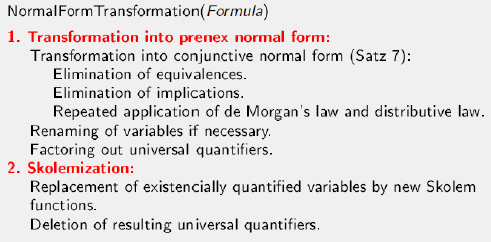
* Skolemization (스콜렘 표준형)
서술 논리에서도 resolution inference rule 을 적용하려 하는데 , 이를 위하여 우리는 먼저 prenex normal 으로 전환하는 방법을 배웠다 . 이는 모든 한정사(quantifier) 가 formula 의 맨 앞으로 이동된 형태의 formula 이다
Prenex normal form 에서 우리는 한정사를 제거하려고 한다 . 먼저 existential quantifier 을 제거하려 한다 .
이런 방법을 Skolemization 이라고 한다 . Skolemization 은 아래의 existential quantifier 식이 disjunction으로 표현된 식과 같으므로 만약 우리가 어떤 상수 Ai 를 안다면 비록 원래 formula 가 skolemization 한 후의 formula, 즉 p(Ai) 가 의미론적으로 동등하지 않을지라도 원래 formula 의 참값은 그대로 유지시킬 수 있겠다 .
이러한 과정을 skolemization 이라고 한다
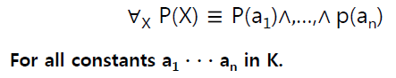
=> For all constants a
1 · · · a n in K.
∃X P(X) ≡P(A1 )v … v p(An) 와 같이 existential quantifier 변경하는 것을 Skolemization 이라고 한다.

Skolemization 과정 중에서 제거하려는 existential quantifier 의 변수가 universal quantifier 에서 사용하는 변수와 관계가 생기면 , 즉 universal quantifier scope 안에 있으면 단순 상수 term 을 사용할 수 없으며 , 그 universal quantifier 에서 사용하는 변수들의 function term, skolem function term 으로 사용되어야 한다 . 이 때 universal quantifier 변수와 관련이 없는 경우는 단순 상수로 skolem constant 라고 불린다 . 이 때 사용되는 skolem constant, function symbol 등은 ontology 에 사용한 심볼들과 이름이 달라야 한다
마지막 단계로 universal quantifier 를 제거하기 위하여는 사용되는 변수들의 이름 역시 전에 사용된 심볼과 중복되어 사용될 수 없다 . 또한 universal quantifier 가 영향은 미치는 즉 scope 내에서는 같은 변수 이름이지만 , 이를 벋어 나면rename 하여 다른 변수 이름을 사용해야 한다.
Example 1.

=> existential quantifier를 function term으로 변경하고,
rename을 통해 universal quantifier를 지우면 Prenex normal form이 완성된다.
Example 2.

=> existential quantifier를 n0 값인 function term으로 변경하고,
n0의 argument로 ε을 넣어 n0( ε) 완성 후 universal quantifier를 지우면 Prenex normal form이 완성된다.
Example 3.

=> 위 식의 Prenex normal form 형태는 다음과 같다.

=> 이후 위에서 나온 식에 negation을 불인다.
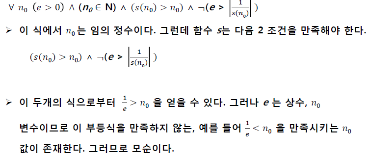
=> counter example을 찾을 수 있으므로 위 식은 contradiction이다.
proof-by-contradiction으로 lim(1/n), n=∞을 증명한 과정이다.
Example 4.
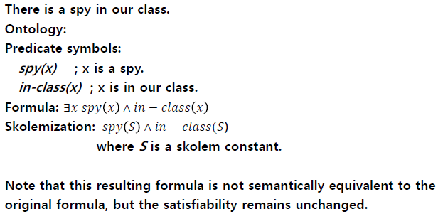
=> universal quantifier가 existential quantifier 앞에 존재하지 않으므로,
skolem constant인 S로 표현한다.
=> 바뀐 formula는 원래의 formula와 equivalent 하지 않지만,
satisfiability 즉, 참 값은 그대로 유지가 된다.
* Program Scheme
명제 논리에서 sound & complete 한 theorem prover, 즉 임의 formula A 에 대여 KB┣ p A if and only if KB ╞ A 를 만족하는 프로그램 p 가 존재한다 .
한 가지 방법으로 resolution refutation 방법을 사용하여 만들 수 있다 . 복잡도는 NP Hard( 이는 NP Complete 와 거의 같은 수준 임 이지만 늘 답을 할 수 있는 즉 알고리즘이 존재하였다 그러면 서술 논리에서도 이러한 프로그램 (universal 이 존재할까
이제 Gödel Completeness theorem 을 배우게 된다 . 이 정리는 컴퓨터 혹은 서술 논리의 입장으로 생각하면
모든 참인 formula 를 증명할 수 있을까 , 즉 sound & complete theorem prover 가 존재하는가에 대한 질문으로 재해석하여 볼 수 있다 . 답은 Gödel 이 증명한 것처럼 가능하다.

=> correctness and completeness 할 경우에 항상 증명이 가능한 알고리즘이 존재한다.
서술 논리에서도 sound & complete theorem prover 가 존재하지만 formula 가 참인 경우는 늘 답을 줄 수 있지만 거짓인 경우는 가끔이지만 답을 주지 못하고 영원히 loop 를 돌 수도 있다 . 이 것을 Gödel 의 incompleteness theorem 에서 증명하고 있다 . 이러한 문제는 컴퓨터 Society 에서 “Halting Problems" 라고 부르기도 한다 . 그러므로 서술 논리에서는 늘 답을 할 수 있는 알고리즘은 존재하지 않는다.
늘 답을 찾아 낼 수 있는 문제를 Decidable Problem 이라고 하며 이를 해결할 수 있는 프로그램을 알고리즘이라고 한다. Halting problem 처럼 답이 참인 경우 답을 늘 주지만 거짓인 경우 답을 주지 못할 수 있는 문제를 Semi decidable Problem 이라고 한다 . 서술 논리에서 sound & complete theorem prover 는 바로 이런 영역에 속하는 문제이다.
- Gödel incompleteness theorem

=> formula 가 참일 때 항상 증명이 가능하다.
=> formula 가 참이 아닐 때 증명을 못하는 경우가 발생한다.
* Inference rules
Example 5.

=> 명제 논리에서는 Modus ponens 를 바로 적용하면 되지만,
서술 논리에는 universal quantifier가 존재하므로 universal quantifier를 제거 후에 Modus ponens를 적용 할 수 있다.
Example 6.
The calculus of the above two rules (MP and ) is sound ,
but not complete.
Why not?
We can simply find a count example:
Given
KB 𝐴𝑥⇒𝐵𝑥,𝐴(𝑎)∨𝐵(𝑎)},
Prove KB ╞ 𝐵(𝑎)
Of course, KB ╞ 𝐵(𝑎) is true
However, using the only two rules, we cannot prove it.
=> Modus ponens는 sound는 하지만 complete 하지는 않다.
* Correctness(Soundness)

* Resolution

=> resolution 하여 empty close를 만들 수 있으므로 증명이 가능하다.
* Unification

서술 논리에서는 변수와 universal quantifier 가 사용된다 . 변수에는 세상의 객체를 가리키는 term 으로 대체될 수 있다. 이렇게 대체되는 process 를 unification 이라고 한다 Universal quantifier 는 전에 배운 대로 다음과 같은 의미론이 적용될 수 있다. 따라서 inference rule 을 적용할 때 unification 을 수행한 결과를 사용할 수 있다.
Example 7.

=> know(x,x) 에는 x에 John을 넣어야 할지 Mary를 넣어야 할지 알지 못하므로 nil이다. (false)
=> know(John,Mary) 의 경우 변수는 없지만, Match가 되므로 unifiable 하다. (true)
Example 7.

=> unification process도 재귀적인 process이다.
=> unification process는 대부분의 case에서 빠르다.
Example 8.

* General Resolution rule for predicate logic

=> Resolution rule은 sound 하지만, complete 하지 않다.
Example 8.

=> 위 예는 Russell의 paradox 이다.
=> "Resolution rule은 sound 하지만, complete 하지 않다 ." 의 counter example이다.
* Factorization
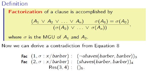
=> unification process가 필요한 경우에는 순수하게 resolution 으로는 안된다.
=> factorization을 통해 위 Example 8번이 complete 하다는 것을 증명할 수 있다.
* Transform to CNF in Predicate Logic
Example 9.
CNF for first order logic: similar to the propositional case.
Ex) ∀x [∀y Animal(y)⇒Loves(x,y)]⇒[∃y Loves(y,x)]
1. Eliminate implications:
∀x ¬ [∀y ¬Animal(y)∨Loves( x,y )]∨[∃y Loves(y,x)]
2. Move ¬ inwards:
¬∀x P becomes ∃x ¬P
¬∃x P becomes ∀x ¬P
∀x [∃y ¬(¬Animal(y)∨Loves(x,y))]∨[∃y Loves(y,x)]
∀x [∃y ¬¬Animal(y)∧¬Loves(x,y)]∨[∃y Loves(y,x)]
∀x [∃y Animal(y)∧¬Loves(x,y)]∨[∃y Loves(y,x)]
3. Standardize(Rename) variables:
∀x [∃y Animal(y)∧¬Loves(x,y)]∨[∃z Loves(z,x)]
4. Skolemize
∀x [Animal(F(x))∧¬Loves(x,F (x))]∨Loves(G(x),x)
5. Drop universal quantifiers:
[Animal(F(x))∧¬Loves( x,F (x))]∨Loves(G(x),x)
6. Distribute ∨ over ∧:
[Animal(F(x)) ∨ Loves(G(x),x) ] ∧[¬Loves(x,F (x))∨Loves(G(x),x)]
Example 10.
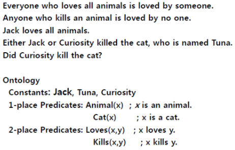
=> Formalization

=> Transform to CNF

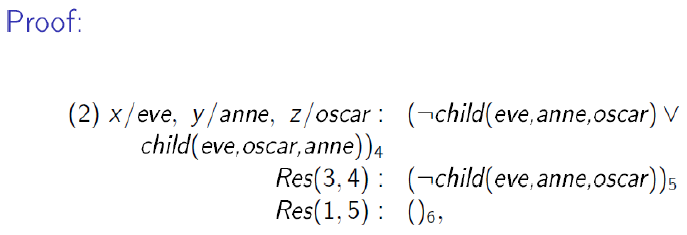
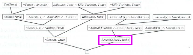
=> A resolution proof that Curiosity killed the cat.
Notice the use of factoring in the derivation of the clause Loves(G(Jack), Jack).
* Knowledge Engineering
Knowledge Engineering 이라 함은 인간 전문가의 지식을 컴퓨터 내에 저장하여 마치 인간 전문가가 하는 역할을 담당할 수 있도록 하는 일련의 process 이다 . 이는 마치 문제가 주어지면 이를 해결하기 위하여 프로그램을 작성하는 것과 유사하다고 할 수 있다.
다만 기존의 컴퓨터 프로그래밍을 통하여 문제를 해결하는 방법은 대부분 문제 해결을 위한 알고리즘을 사람이 찾아 내어 프로그래밍하여 해결하는 소위 절차적 접근 (Procedural 이라고 하는 방식이다 . 이러한 방식은 문제가 바뀌면 새로운 알고리즘을 다시 찾아 프로그램을 다시 하는 방식이 된다 . 물론 소프트웨어 재사용이란 관점에서 모듈화 하여 재사용의 비율을 높이는 기법들도 이미 많이 연구되어 왔지만 , 근본적으로 어려운 문제이다.
반면 인공지능의 지식표현과 추론이라는 관점에서는 지식베이스와 추론엔진의 개념을 통하여 지식을 지식베이스에 축적하여 문제가 바뀌어도 지식베이스에 있는 지식과 추론엔진을 통하여 새롭게 알고리즘을 만들지 않고 단순히 지식을 추가함으로 그 문제를 해결하고자 하는 방식이다.
이러한 접근 방식을 선언적 방식 (Declarative 이라고 부른다 . 이 경우 지식을 표현하는 언어로 서술 논리가 이론적으로 최강의 언어라고 할 수 있다 . 다만 사용성의 편의를 위하여 보다 구조화된 고급지식표현 언어들이 지식표현 및 추론 시스템으로 사용되고 있다.
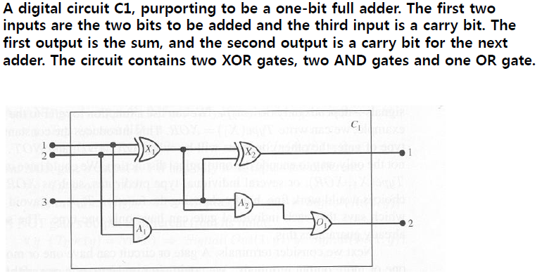
이러한 지식공학 프로세스를 살펴보기 위하여 1 bit Full Adder 의 회로를 인용하다 (Refer to Modern Approach to AI) 1 bit Full Adder 는 3 개의 input bits, x, y, c 가 주어지면 x+y 를 하는데 전에 넘어 오는 carry bit c 를 고려여 x+y+c 를 계산하고 그 결과를 2 개의 output bits s 과 c 이 나오게 된다 . s 는 결과 bit 이고 c 는 carry bit 이다 .
예를 들어 x=1, y=0, c=0 이면 s=1, c=0 이 된다 . x=1, y=1, c=0 이면 s=0, c=1 이 된다 . x=1, y=0, c=1 면 s=0, c=1 이 된다 . 이러한 1 bit Full Adder 32 개를 연결해 만들면 32 bit 짜리 더하기 계산 회로를 만들 수 있다.
* Knowledge Engineering in First-Order Logic
Knowledge engineering process
1. Identify the task
2. Assemble the relevant knowledge: knowledge acquisition process is needed.
3. Decide on a vocabulary of predicates, functions, and constants.(Ontology of the domain) Note that ontology means a particular
theory of the nature of being or existence.
4. Encode general knowledge about the domain.
5. Encode a description of the specific problem instance.
6. Pose queries to the inference procedure and get answers.
7. Debug the knowledge base.
* The electronic circuits domain
Example 11.
이러한 문제를 해결하기 위하여 수집된 지식을 만약 서술 논리로 표현하고자 하면 먼저 ontology 를 정해야 한다 . Ontology 를 정하는 것은 문제에 따라 달라질 수 있기 때문에 미리 철저하게 계획에서 정하는 것이 좋다
예를 들어, 이 회로에서 사용하는 gate 가 3 가지 OR, AND, XOR 가 있는데 이러한 심볼을 상수로 사용할까 ? 사용한다면 회로에 나오는 X1 gate 를 XOR gate 라고 말할 때 어떻게 할까 ? Type 이라는 심볼을 function 으로 사용하면Type(X1)=XOR 라고 표현하게 되고 , 만약 predicate symbol 로 사용하면 Type(X1, XOR) 으로 표현하게 될 것이다 . 아래에서는 function symbol 로 사용하였다
그 외에도 In, Out 은 2 place function symbol 로 사용하여 gate 의 몇 번째 input/output 인지를 가리키고 , Connected 는 2 place predicate symbol 로 사용하여 그 회로 혹은 gate 가 연결되었다는 관계를 나타내고 있다 . 또한 Signal 은 1 place function symbol 로 회로의 지점 , 즉 terminal 의 값 (0 혹은 1) 을 나타낸다
1. Identify the task: Figure in the next slide
2. Assemble the relevant knowledge: Digital circuits are composed of wires and gates. Signals flow along wires to the input terminals of gates, and each gate produces a signal on the output terminal that flows along another wire. There are four type of gates: AND, OR, XOR, and NOT.
3. Deciding on a vocabulary: circuits, terminal, signals, and gates, some constants X 1 , X 2 , and so on. Function vs predicate: Type(X 1 ) = XOR or Type(X 1 , XOR). X 1 In 1 or In(1, X1)? Connected(Out(1,X 1 ), In(1,X 2)
4. Encode general knowledge of the domain
1.∀t 1 ,t 2 Connected(t 1 ,t 2 )⇒Signal(t 1 )=Signal(t 2)
2.∀t Signal(t)=1 V Signal(t)=0; 1 ≠ 0
3.∀ t 1 ,t 2 Connected(t 1 ,t 2 )⇔ Connected(t 2 ,t 1 )
4.∀g Type(g)=OR ⇒ Signal(Out(1,g))=1⇔∃n Signal( n,g ))=1
5.∀g Type(g)=AND ⇒ Signal(Out(1,g))=0⇔∃n Signal( n,g ))=0
6.∀g Type(g)=XOR ⇒ Signal(Out(1,g))=1⇔Signal(In(1,g)) ≠ Signal(In(2,g))
7.∀g Type(g)=NOT ⇒ Signal(Out(1,g)) ≠ Signal(In(1,g))
5. Encode the specific problem instance ( 회로 C1 에 대한 표현
Type(X 1 ) = XOR Type(X 2 ) = XOR
Type(A 1 ) = AND Type(A 2 ) = AND
Type(O 1 ) = OR
Connected(Out(1,X 1 ),In(1,X 2 )) Connected(In(1,C 1 ),In(1,X 1 ))
Connected(Out(1,X 1 ),In(2,A 2 )) Connected(In(1,C 1 ),In(1,A 1 ))
Connected(Out(1,A 2 ),In(1,O 1 )) Connected(In(2,C 1 ),In(2,X 1 ))
Connected(Out(1,A 1 ),In(2,O 1 )) Connected(In(2,C 1 ),In(2,A 1 ))
Connected(Out(1,X 2 ),Out(1,C 1 )) Connected(In(3,C 1 ),In(2,X 2 ))
Connected(Out(1,O 1 ),Out(2,C 1 )) Connected(In(3,C 1 ),In(1,A 2))
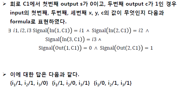
6. Pose queries to the inference procedure What combinations of inputs would cause the first output of C 1 (the sum bit) to be 0 and the second output of C 1 (the carry bit) to be 1?
∃i 1 ,i 2 ,i 3 Signal(In(1,C 1 ))=i 1 ∧ Signal(In(2,C 2 ))=i 2 ∧ Signal(In(3,C 1 ))=i 3 ∧Signal(Out(1,C 1 ))=0∧Signal(Out(2,C 1 )=1
There are three substitutions:
{i 1 /1, i 2 /1, i 3 /0} {i 1 /1, i 2 /0, i 3 /1} {i 1 /0, i 2 /1, i 3 /1}
아주대학교 정보통신대학원 김민구 교수님의 인공지능 강의를 바탕으로 작성하였습니다.
학습 목적으로 포스팅 합니다.
'Artificial Intelligence' 카테고리의 다른 글
| Limitations of Logic (0) | 2020.09.30 |
|---|---|
| 서술논리 ① (0) | 2020.09.23 |
| 명제논리 (2) | 2020.09.12 |